import pandas as pd
import numpy as np
import matplotlib.pyplot as plt
from pymech.dataset import open_mfdataset


df = pd.read_csv("LM_Channel_5200_mean_prof.txt", sep=r'\s+', comment='%')
df
| y_over_delta | y_plus | U | dU_dy | W | P | |
|---|---|---|---|---|---|---|
| 0 | 0.000000 | 0.000000 | 0.000000 | 1.000000 | 0.000000 | 0.000000e+00 |
| 1 | 0.000014 | 0.071102 | 0.071102 | 0.999986 | -0.000011 | -4.717272e-09 |
| 2 | 0.000042 | 0.216250 | 0.216244 | 0.999947 | -0.000034 | -3.851045e-07 |
| 3 | 0.000085 | 0.438384 | 0.438355 | 0.999819 | -0.000069 | -6.055743e-06 |
| 4 | 0.000143 | 0.740447 | 0.740306 | 0.999379 | -0.000117 | -4.477271e-05 |
| ... | ... | ... | ... | ... | ... | ... |
| 763 | 0.991022 | 5139.336002 | 26.574682 | 0.000026 | -0.006544 | -4.790325e-01 |
| 764 | 0.993017 | 5149.682732 | 26.574923 | 0.000020 | -0.006553 | -4.789895e-01 |
| 765 | 0.995012 | 5160.029605 | 26.575104 | 0.000015 | -0.006562 | -4.789556e-01 |
| 766 | 0.997007 | 5170.376581 | 26.575224 | 0.000009 | -0.006568 | -4.789319e-01 |
| 767 | 0.999002 | 5180.723618 | 26.575284 | 0.000003 | -0.006571 | -4.789196e-01 |
768 rows × 6 columns
Here:
y_over_delta: $y/\delta$ Grid point in wall-normal direction, Normalized by channel half width
y_plus : Grid point in wall-normal direction
U : Mean profile of streamwise velocity (normalized with $u^*$)
dU/dy : Derivative of U in wall-normal direction
W : Mean profile of spanwise velocity
P : Mean profile of pressure
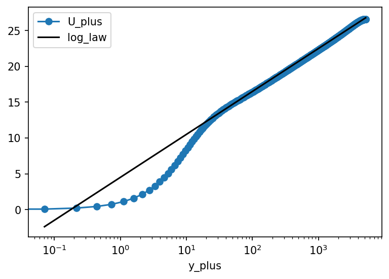
kappa = 0.384
u_star = 1.
B = 4.5
y0 = np.exp(-kappa * B)
df["U_plus"] = df.U / u_star
df["log_law"] = np.log(df.y_plus / y0) / kappa

# Plot
plt.rc("figure", dpi=150)
ax = df.plot("y_plus", "U_plus", marker='o')
df.plot("y_plus", "log_law", ax=ax, color="k")

ax.set(xscale="log")
print(f"{y0}")
/home/x_ashmo/.conda/envs/snek/lib/python3.7/site-packages/pandas/core/series.py:679: RuntimeWarning: divide by zero encountered in log
  result = getattr(ufunc, method)(*inputs, **kwargs)
0.17763933359513495
y0 / df.y_plus.max()
3.4288517720901714e-05
Comparison
cd /proj/bolinc/users/x_ashmo/channel_tests/abl_ch-channel_mixing_len_14x4x7_V6.283x2.x3.142_2021-04-08_15-23-17
/proj/bolinc/users/x_ashmo/channel_tests/abl_ch-channel_mixing_len_14x4x7_V6.283x2.x3.142_2021-04-08_15-23-17
spatial_means = pd.read_csv("spatial_means.txt", sep=r'\s+')
spatial_means.tail()
| it | t | ux_avg | ez_avg | u_star_avg | u_star_max | dpdx_avg | dpdy_avg | |
|---|---|---|---|---|---|---|---|---|
| 11994 | 239900 | 1499.5 | 1.0 | 0.000521 | 0.026400 | 0.047683 | -6.2832 | -6.2832 |
| 11995 | 239920 | 1499.6 | 1.0 | 0.000521 | 0.026400 | 0.047697 | -6.2832 | -6.2832 |
| 11996 | 239940 | 1499.7 | 1.0 | 0.000520 | 0.026399 | 0.047718 | -6.2832 | -6.2832 |
| 11997 | 239960 | 1499.8 | 1.0 | 0.000520 | 0.026399 | 0.047734 | -6.2832 | -6.2832 |
| 11998 | 239980 | 1499.9 | 1.0 | 0.000519 | 0.026398 | 0.047754 | -6.2832 | -6.2832 |
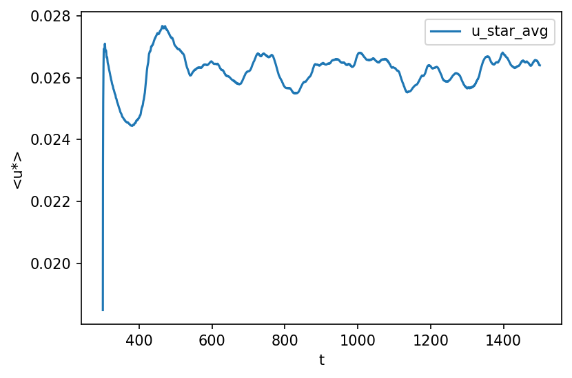
ax = spatial_means.plot("t", "u_star_avg")
ax.set(ylabel="<u*>")
[Text(0, 0.5, '<u*>')]
ds = open_mfdataset("stsabl0.f007??")
dss = ds.mean(("x", "z", "time"))

U = (dss.s01**2 + dss.s02**2) ** 0.5

tau = (dss.s47**2 + dss.s50**2)**0.5
u_star = tau.isel(y=0)**0.5
float(u_star)
0.06669730128082715
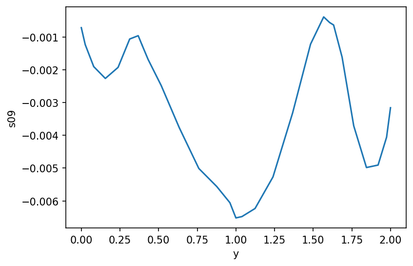
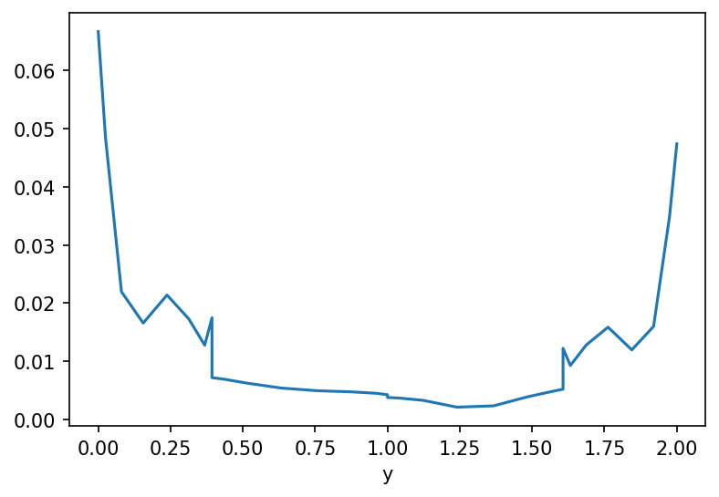
dss.s09.plot()
[<matplotlib.lines.Line2D at 0x7f8664fd23d0>]
tau = (dss.s47**2 + dss.s50**2)**0.5
(tau**0.5).plot()
[<matplotlib.lines.Line2D at 0x7f8664e47190>]
u_star = spatial_means[spatial_means.t > 550].u_star_avg.median()
u_star
0.026367
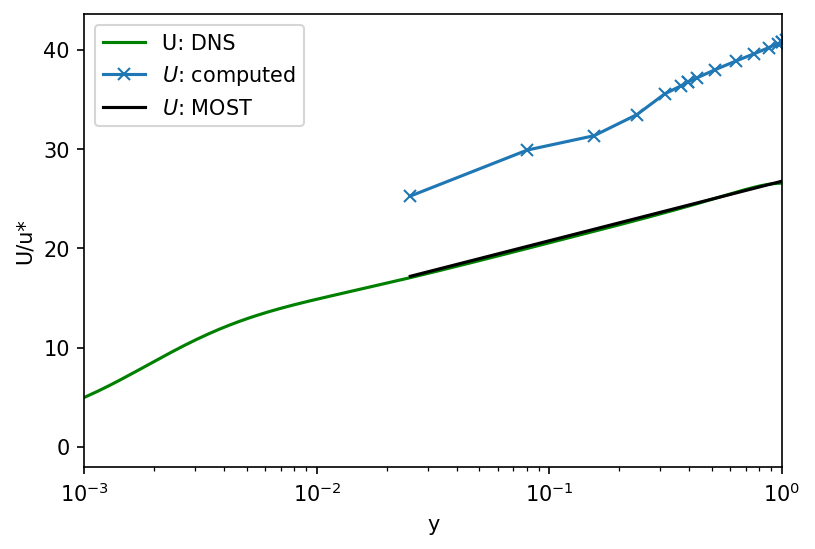
kappa = 0.384
z = ds.y # + 1e-1
z0 = 3.4289e-5
U_most =  u_star / kappa * np.log(z / z0)

fig, ax = plt.subplots(dpi=150)
df.plot("y_over_delta", "U_plus", color="g", ax=ax, label="U: DNS")


ax.plot(z[1:], (U / u_star)[1:], marker="x", label=r"$U$: computed")
ax.plot(z[1:], (U_most / u_star)[1:], color="k", label=r'$U$: MOST')
ax.set(xscale="log", xlabel="y", ylabel="U/u*", xlim=(1e-3, 1))
ax.legend()
/home/x_ashmo/.conda/envs/snek/lib/python3.7/site-packages/xarray/core/computation.py:604: RuntimeWarning: divide by zero encountered in log
  result_data = func(*input_data)
<matplotlib.legend.Legend at 0x7f86650c3090>
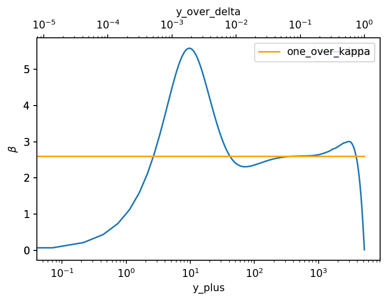
The indicator function
Theoretically $$\frac{\partial U^+}{\partial y^+} = \frac{1}{\kappa y^+}$$ in the log-law region to check this we use the indicator function $$\beta (y^+) = y^+ \frac{\partial U^+}{\partial y^+}$$
df["beta"] = df.y_plus * df.dU_dy
df["one_over_kappa"] = 1 / kappa

ax = df.plot("y_plus", "beta")
ax_top = ax.twiny()
df.plot("y_over_delta", "one_over_kappa", color='orange', ax=ax_top)
ax.set(ylabel=r"$\beta$", xscale="log")
ax_top.set(xscale="log")
ax.legend()
<matplotlib.legend.Legend at 0x7f8664411d90>